Mechatronic layer

Introduction

The ARTOF framework is ideally integrated during the development of a new robot platform, but can also be integrated afterwards. The mechatronic layer requires a custom implementation tailored to the specific vehicle configuration, selected components, and the platform’s safety requirements.

Requirements

The minimal hardware requirements to perform steering guidance are:

1. Safety: The implementation of the mechatronic layer is responsible for all the platform’s safety features in accordance with national legislation. This implementation is machine dependent and is not provided by the ARTOF framework.

2. Programmable Logic Controller: A PLC interfaces with all the actuators and sensors on the platform. At a minimum, it must implement the inverse and direct kinematic models to ensure correct control of the steering and driving actuators.

   • Example components: Siemens S7-1200 and Siemens S7-1500 series

3. Steering angle control: The steering angle needs to be controlled by the PLC.

   • For hydraulic steering, this can be done using a hydraulic steering block.

   • For electric steering, this can be done by controlling the motor drive.

   • Example components: Raven® RS1

4. Steering angle feedback: The PLC needs to monitor the steering angle to enable closed-loop steering control.

   • For Ackerman steering robots, this can be done with an inductive angle sensor on the steering rack.

   • For 4WD4WS steering robots, all the wheel angles need to be measured, which can also done using inductive angle sensors.

   • Example components: Multiprox® RI360P1-QR20-LU4X2-H1141

5. Velocity control: The driving velocity needs to be controlled by the PLC.

   • For hydraulic traction, this can be done by controlling the swash plate with an electric actuator.

   • For electric traction, this can be done by setting the motor drives to velocity control.

   • An electronic analogue paddle can be used for robots that enabled paddle velocity control for the driver.

6. Velocity feedback: The PLC needs to monitor the driving velocity to enable closed-loop velocity control.

   • For robots with hydraulic transmission, this can be done by a rotary encoder and two interlocking cogs.

   • For robots with electrical transmission, this can be done by reading the hall sensor, sin/cos encoder, etc.

Additional requirements to operate a robot platform:

1. Hitch control: The hitches need to be controlled by the PLC.

   • For hydraulic hitches this can be done using electric valves.

2. Hitch angle feedback: The PLC needs to monitor the hitch angles to enable closed-loop hitch height control.

   • If no actuator feedback is available, this can be done using inductive angle sensors.

   • Example components: Multiprox RI360P1-QR20-LU4X2-H1141

Note

All safety measures must be implemented within the mechatronic layer. The operational layer does not include safety features and should only be used on products approved for autonomous operation in accordance with national legislation.

Safety state diagram

For more information on the safety state diagram, we refer to the paper <Coming soon>.

Kinematic model

Introduction

Note

Abbreviation used:

1. longitude (lng), latitude (lat)

2. front (f), rear (r), so fr (front-right)

3. angular velocity (\(\omega\)), steering angle (\(\epsilon\))

The direct kinematic model describes the actual platform’s motion by the velocity vector \(\boldsymbol{v_a} = (v_x, v_y, \omega_z)\) based on the actuators feedback e.g. \(\omega_{wheel,rr}\), \(\omega_{wheel,rl}\), \(\epsilon_{f}\), \(\epsilon_{fl}\), etc., depending on the vehicle configuration.

The inverse kinematic model does the opposite and starts from the required motion or velocity vector \(\boldsymbol{v_r} = (v_{lng}, v_{lat}, \omega_z)\) to calculate the position or velocities of the actuators.

Kinematic means no external forces are incorporated in this model to come to this motion. A model where the external forces are incorporated is called a dynamic model.

The kinematic model is integrated into the mechatronic layer, making the operational layer independent of the vehicle configuration. An essential part of the mechatronic-operational layer interface is the infterface with the actual and required velocity vector.

• The interface with the actual velocity vector \(\boldsymbol{v_a}\) is described in the Redis variables plc.monitor.navigation.velocity.longitudinal, plc.monitor.navigation.velocity.lateral, plc.monitor.navigation.velocity.angular.

• The interface with the required velocity vector \(\boldsymbol{v_r}\) is described in the Redis variables plc.control.navigation.velocity.longitudinal, plc.control.navigation.velocity.lateral, plc.control.navigation.velocity.angular.

The book Vehicle Dynamics by Reza N. Nazar contains much information about vehicle kinematics and dynamics.

Jazar, R. N. (2008). Vehicle dynamics (Vol. 1). Berlin/Heidelberg,
Germany: Springer.

Four-wheel-drive four-wheel-steer (4WD4WS)

Figure 1 was used to derive the kinematic model of a four-wheel-drive, four-wheel-steer (4WD4WS) robot.

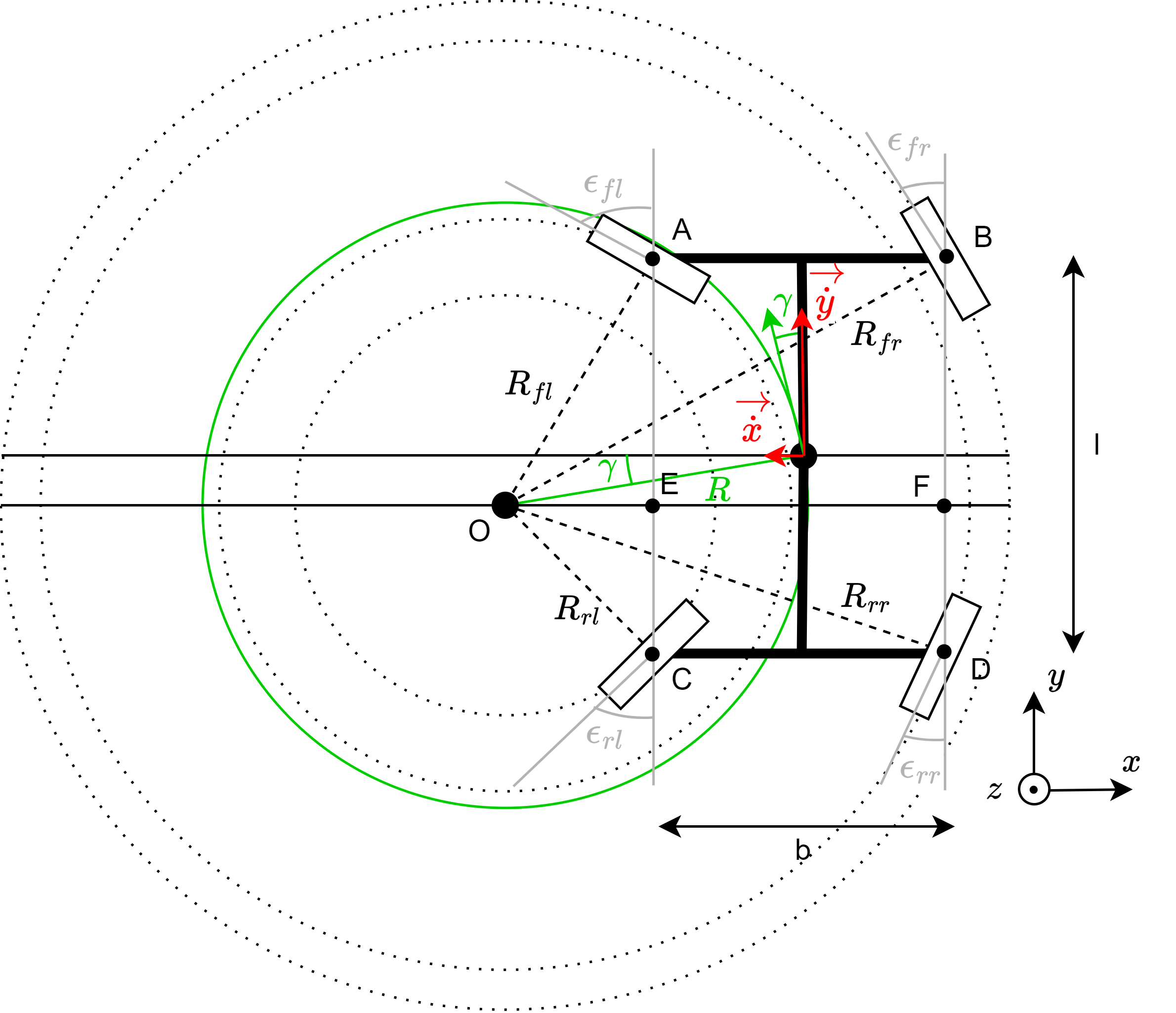
Figure 1. Kinematics 4WD4WS vehicle configuration

For the direct kinematic model

\[f(v_{fl}, v_{fr}, v_{rl}, v_{rr}, \epsilon_{fl}, \epsilon_{fr}, \epsilon_{rl}, \epsilon_{rr}) = (v_x, v_y, \omega_z)\]

The following formulas can be extracted using Figure 1.

\[\begin{split}v_{fl} &= R_{w} \cdot \omega_{w,fl} \\ v_{fr} &= R_{w} \cdot \omega_{w,fr} \\ v_{rl} &= R_{w} \cdot \omega_{w,rl} \\ v_{rr} &= R_{w} \cdot \omega_{w,rr} \\ v_{y} &= \frac{1}{4} \left[ v_{fl} \cdot cos(\epsilon_{fl}) + v_{fr} \cdot cos(\epsilon_{fr}) + v_{rl} \cdot cos(\epsilon_{rl}) + v_{rr} \cdot cos(\epsilon_{rr}) \right] \\ v_{x} &= \frac{1}{4} \left[ v_{fl} \cdot sin(\epsilon_{fl}) + v_{fr} \cdot sin(\epsilon_{fr}) + v_{rl} \cdot sin(\epsilon_{rl}) + v_{rr} \cdot sin(\epsilon_{rr}) \right] \\ \omega_{z} & = \frac{l}{2} \left( \left[ v_{rl} \cdot sin(\epsilon_{rl}) + v_{rr} \cdot sin(\epsilon_{rr}) \right] - \left[ v_{fl} \cdot sin(\epsilon_{fl}) + v_{fr} \cdot sin(\epsilon_{fr}) \right] \right)\end{split}\]

The inverse kinematic model

\[g(v_x, v_y, \omega_z) = (v_{fl}, v_{fr}, v_{rl}, v_{rr}, \epsilon_{fl}, \epsilon_{fr}, \epsilon_{rl}, \epsilon_{rr})\]

First, the points \(\mathrm{A}\) up to \(\mathrm{F}\) indicated in Figure 1, \(\mathrm{R}_{xx}\) were determined.

\[\begin{split}&\left|\mathrm{AE}\right| = \left|\mathrm{BF}\right| = \frac{\mathrm{l}}{2} + \mathrm{R} \sin(\gamma) \\ &\left|\mathrm{EC}\right| = \left|\mathrm{FD}\right| = \frac{\mathrm{l}}{2} - \mathrm{R} \sin(\gamma) \\ &\left|\mathrm{OE}\right| = \mathrm{R} \cos(\gamma) - \frac{\mathrm{b}}{2} \\ &\left|\mathrm{OF}\right| = \mathrm{R} \cos(\gamma) + \frac{\mathrm{b}}{2} \\ &\mathrm{R}_{fl} = \left(\left|\mathrm{AE}\right|^2 + \left|\mathrm{OE}\right|^2 \right)^{\frac{1}{2}} \\ &\mathrm{R}_{fr} = \left(\left|\mathrm{OF}\right|^2 + \left|\mathrm{BF}\right|^2 \right)^{\frac{1}{2}} \\ &\mathrm{R}_{rl} = \left(\left|\mathrm{OE}\right|^2 + \left|\mathrm{EC}\right|^2 \right)^{\frac{1}{2}} \\ &\mathrm{R}_{rr} = \left(\left|\mathrm{OF}\right|^2 + \left|\mathrm{FD}\right|^2 \right)^{\frac{1}{2}}\end{split}\]

Also, we know:

\[\begin{split}&\mathrm{\Delta v}_f = \big| (\mathrm{R}_{fl} - \mathrm{R}_{fr}) \cdot \dot{\mathrm{\theta}} \big| \\ &\mathrm{\Delta v}_r = \big| (\mathrm{R}_{rl} - \mathrm{R}_{rr}) \cdot \dot{\mathrm{\theta}} \big|\end{split}\]

Using the radius \(\mathrm{R}_{xx}\) given the equations above, \(\omega_{w,xx}\) and \(\epsilon_{xx}\) were calculated.

\[\begin{split}& \mathrm{\omega}_{w,fl} = \mathrm{sgn}(\dot{\mathrm{y}})\cdot \big(- \mathrm{sgn}(\dot{\mathrm{\theta}})\,\frac{\mathrm{\Delta v}_f}{2} + v\big) \cdot \frac{2}{\mathrm{D}_w}\\ & \mathrm{\omega}_{w,fr} = \mathrm{sgn}(\dot{\mathrm{y}})\cdot \big( \mathrm{sgn}(\dot{\mathrm{\theta}})\,\frac{\mathrm{\Delta v}_f}{2} + v \big) \cdot \frac{2}{\mathrm{D}_w}\\ & \mathrm{\omega}_{w,rl} = \mathrm{sgn}(\dot{\mathrm{y}})\cdot \big(- \mathrm{sgn}(\dot{\mathrm{\theta}})\,\frac{\mathrm{\Delta v}_r}{2} + v \big) \cdot \frac{2}{\mathrm{D}_w}\\ & \mathrm{\omega}_{w,rr} = \mathrm{sgn}(\dot{\mathrm{y}})\cdot \big( \mathrm{sgn}(\dot{\mathrm{\theta}})\,\frac{\mathrm{\Delta v}_r}{2} + v \big) \cdot \frac{2}{\mathrm{D}_w} \\ & \mathrm{\epsilon}_{fl} = \arctan \left( \frac{\left|\mathrm{AE}\right|}{\left|\mathrm{OE}\right|} \right) \\ & \mathrm{\epsilon}_{fr} = \arctan \left( \frac{\left|\mathrm{BF}\right|}{\left|\mathrm{OF}\right|} \right) \\ & \mathrm{\epsilon}_{rl} = \arctan \left( - \frac{\left|\mathrm{EC}\right|}{\left|\mathrm{OE}\right|} \right) \\ & \mathrm{\epsilon}_{rr} = \arctan \left( - \frac{\left|\mathrm{FD}\right|}{\left|\mathrm{OF}\right|} \right)\end{split}\]

Ackerman steering

Figure 2 is used to derive the kinematic model of an Ackerman vehicle.

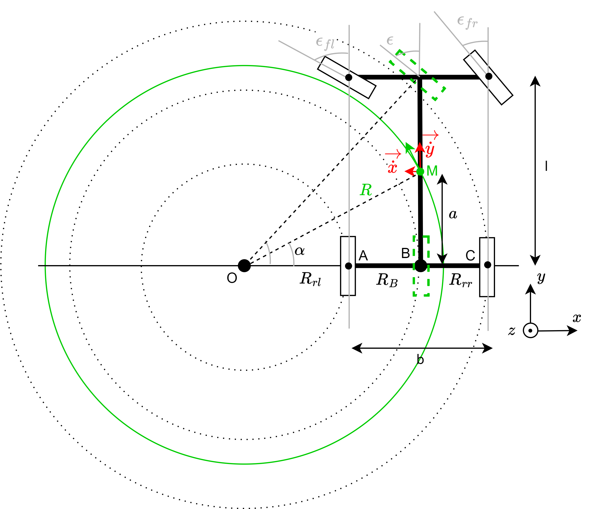
Figure 2. Kinematics Ackerman vehicle configuration, with M as the center of mass.

The four-wheel vehicle model can be reduced to the bicycle model, indicated by the green dot lines in Figure 2. The mass centre (M) will turn on the green circle around the Instanious Center of Rotation (ICR) (point O in Figure 2) with the radius in Equation 1.

(1)\[R = \sqrt{a^2 + l^2 \, \mathrm{cot}^2(\epsilon)}\]

The cot-average Equation 2 and the Ackerman condition in Equation 3 apply in the geometry of the steering rack.

(2)\[\mathrm{cot}(\epsilon) = \frac{\mathrm{cot}(\epsilon_{fl}) + \mathrm{cot}(\epsilon_{fr})}{2}\]

(3)\[\frac{b}{l} = \mathrm{cot}(\epsilon_{fr}) - \mathrm{cot}(\epsilon_{fl})\]

We can find the relation \(\epsilon\) and \(\epsilon_{fl}\) and between \(\epsilon\) and \(\epsilon_{fr}\) by substituting the ackerman condition (Equation 3) into the (Equation 2).

(4)\[\frac{b}{2\,l} = \mathrm{cot}(\epsilon) - \mathrm{cot}(\epsilon_{fl})\]

(5)\[-\frac{b}{2\,l} = \mathrm{cot}(\epsilon) - \mathrm{cot}(\epsilon_{fr})\]

In Figure 2 we can see that the Equations \(\mathrm{tan}(\epsilon) = \frac{l}{R_B}\) and \(\mathrm{tan}(\alpha) = \frac{a}{R_B}\) apply. We can calculate \(\alpha\) in Equation 6.

(6)\[\alpha = \mathrm{atan} \big(\frac{a}{l}\, \mathrm{tan}(\epsilon) \big)\]

By substituting Equation 4 into Equation 6, we find the relation \(\alpha = q(\epsilon_{fl})\) in equation Equation 9.

(7)\[\alpha = \mathrm{atan} \big( \frac{a}{\frac{b}{2} + l\, \mathrm{cot}(\epsilon_{fl})} \big)\]

Assume that we only measure the front-left steering angle \(\epsilon_{fl}\) and the angular velocity of the rear-right wheel \(\epsilon_{rr}\). For small angles in \(\epsilon\), we can assume \(\omega_A = \omega_B = \omega_C\). Consequently Equation 8 applies.

(8)\[\frac{v_{rr}}{R_{rr}} = \frac{v_{y}}{R_{B}}\]

The direct kinematic model

\[f(v_{rr}, \epsilon_{fl}) = (v_x, v_y, \omega_z)\]

We can find the relation \(\epsilon = q(\epsilon_{fl})\) by rearranging Equation 4.

(9)\[\epsilon = \mathrm{acot} \big( \frac{b}{2\,l} + \mathrm{cot}(\epsilon_{fl}) \big)\]

Equation 7 can be used to integrate into the equations of the direct kinematic model below.

\[\begin{split}v_y &= \frac{R_B}{R_{rr}}\,v_{rr} = \frac{R\, \mathrm{cos}(\alpha)}{R\, \mathrm{cos}(\alpha) + \big(\frac{b}{2}\big)}\,v_{rr} \\ v_x &= v_y \, \mathrm{tan}(\alpha) \\ v &= \sqrt{v^2_x + v^2_y} \\ \omega_z &= \frac{v}{R}\end{split}\]

The inverse kinematic model

\[g(v_x, v_y, \omega_z) = (v_{rl}, \epsilon_{fr})\]

We can determine \(\epsilon\) using the green circle’s radius in Equation 1.

(10)\[\epsilon = \mathrm{acot}\bigg( \frac{\sqrt{\big( \frac{v}{\omega} \big)^2 - a^2}}{l^2} \bigg)\]

By rearranging Equation 4 and by assuming the angular velocity equality (Equation 5) we can determine the inverse kinematic model.

\[\begin{split}\epsilon_{fl} &= \mathrm{acot}\bigg( cot(\epsilon) - \frac{b}{2\,l}\bigg) \\ v_{rr} &= \frac{R_{rr}}{R_B} \, v_y = \frac{R + \big(\frac{b}{2}\big)}{R}\,v \, \mathrm{cos}(\alpha)\end{split}\]

Skid steering

Figure 3 was used to derive the kinematic model of a skid steering robot.

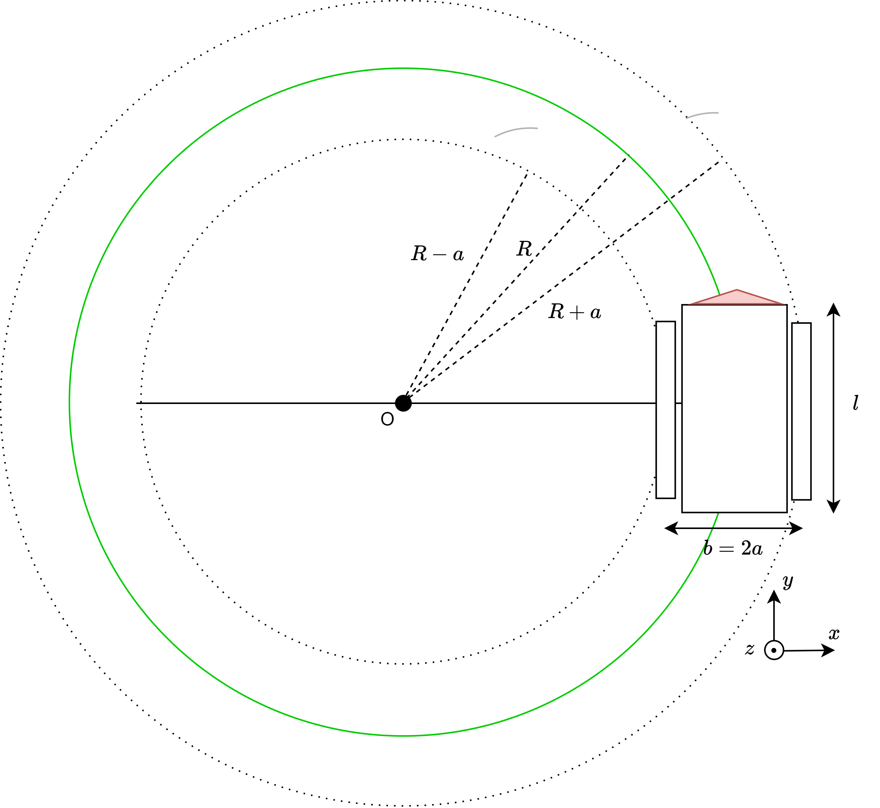
Figure 3. Kinematics skid steering vehicle configuration

The direct kinematic model

\[f(v_{l}, v_{r}) = (v_x, v_y, \omega_z)\]

\[\begin{split}v_x &= 0 \\ v_y &= \frac{v_r + v_l}{2} \\ \omega_z &= \frac{v_r - v_l}{b}\end{split}\]

The inverse kinematic model

\[g(v_x, v_y, \omega_z) = (v_{l}, v_{r})\]

Imagine the robot driving in a circle. All parts of the robot move with the same rotational velocity around the ICR (point O in Figure 3), consequently the equality \(\omega = \omega_r = \omega_l\).

\[\begin{split}\omega_z &= \frac{v}{R} = \frac{v_l}{R-a} = \frac{v_r}{R+a} \\ \Leftrightarrow v_l &= \frac{v}{\frac{R}{R-a}} = \frac{2v}{\frac{R+a}{R-a} + 1} \,\,\, , \,\,\, v_r = \frac{v}{\frac{R}{R+a}} = \frac{2v}{\frac{R-a}{R+a} + 1}\end{split}\]